Selecting the correct level of parallelization for CFD simulations
In this blog, we will look at how to select the level of parallelization for a CFD simulation on the cloud. To do so we will use the example of the Weather Research and Forecast (WRF) model, which is a type of Computational Fluid Dynamics (CFD) simulation. Our experiments will be run using c6i and c5d instances from Amazon Web Services (AWS). But first let’s start with some background on how a CFD simulation is parallelized.
How are CFD simulations parallelized?
CFD simulations works by discretizing space into thousands, or sometimes millions of cells. An iterative method is then used to solve the Navier-Stokes fluid equations over this domain. To achieve large scale parallelization in CFD, the domain can be broken down into multiple subdomains. Each core takes charge of executing the computations over one of these subdomains. Cores responsible for neighboring subdomains exchange the required information using MPI protocols. It becomes clear then that both the computational speed of the cores as well as their bandwidth ability are crucial to achieve good large scale parallelization.
What metrics do we use to measure parallelization?
Before we can talk about parallelization it is important to understand some key metrics that relate to it.
The first of these is the Scale-Up (SC). This metric measures the improvement gained from running a problem on multiple cores when compared to running it on a single core. For cores, it can be calculated as follows:
![]()
Having defined the Scale-Up, we can talk about the efficiency. This is simply equal to the Scale-Up divided by the number of processors used. Optimally, efficiency should always be as close to 100% as possible, although this is not possible for large scale parallelization. It can also be interesting to compare the measured efficiency to the theoretical efficiency, as defined by Amdahl’s Law.
The hardware used
In this blogpost the instances we are going to compare are the c5d and c6i types on the Amazon EC2 cluster.
The c5d instances, which are a bit older, are comprised of custom 2nd generation Intel Xeon Scalable Processors. They feature a an all core Turbo frequency of 3.6Hz. For an additional hourly fee, they can also be launched as EBS-optimized instances enabling them to use a higher bandwidth when communicating using the MPI protocol.
The newer c6i instances also use Intel Xeon Scalable Processors, this time 3rd generation. The frequency is listed at 3.5Hz and they can also be launched with the EBS-optimized option.
Execution time vs cores
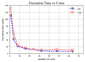
Now lets look at some data. We run a WRF simulation with 1.6 million cells and approximately 1,500 timesteps and collected some execution results.
The first thing we notice is that as expected the execution time goes down as the number of cores grows. This effect is less pronounced as the number of cores continues to go up. As the core number goes up, the computation time to solve the grid becomes lower as each core is responsible for less and less calculations. However, at a certain point this benefit starts being negated by the idling time which the cores need to exchange the necessary messages before performing the next iteration. The more the cores, the more the larger the size of the messages.
How many cores is enough cores?
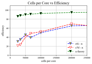
When deciding the optimal amount of cores. It could be interesting to look at Amdahl’s Law and calculate the theoretical efficiency. As seen in the figure, this would suggest that it is possible to achieve a very high level of parallelization with reasonable accuracy. In practice however we notice a steady drop in the parallel efficiency as more cores are added. There is a sharp drop when each core is responsible for less than 50,000 compute nodes. This is a good rule of thumb to remember.
Does fastest always mean better?
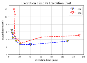
Finally lets also look at a second execution metric, namely the execution cost. Although it might be tempting to run a model many cores and achieve impressive execution times, the cheapest execution options here are the ones corresponding to approximately 20min of execution time. Comparing this with the first figure shown, this means less than 10 cores where used for the cheapest execution. Selecting cores should be thought of as a multi-objective optimization problem in which your own priorities (how important is cost and how important is execution time to your project) need to weight in to your final decision. It is also worth noting here that renting modern infrastructure is key. Notice that the 3rd generation Intel CPUs of the c6i instances outperformed the 2nd generation cores of the c5d instances.
Conclusions
Every case of CFD is different. In the end the safest option is always to run some benchmarking tests on your grid and select your hardware appropriately. However some rules of thumb that were outlined in this blog can help you along. Remember that a value of less than 50,000 cells/core is rarely efficient and that execution speed isn’t always everything. Finally, always try to rent modern infrastructure as the better performance often makes up for the higher cost/hr.